Introduction to Julia by TV denoising

In this post, we implement color-image TV denoising in the Julia programming language.

Total Variation Color Image Denoising

The TV-denoising model can be motivated by wanting to approximate a clean image as piecewise constant. As such, the desired image will have a sparse gradient, $\nabla \mathbf{x}$. We can approximate the gradient to first order by a finite difference scheme, $\nabla \mathbf{x} \approx \mathbf{D}\mathbf{x}$, with $(\mathbf{D}\mathbf{x})[i] = \mathbf{x}[i]-\mathbf{x}[i-1]$.

We then formulate the TV-denoising problem as

and which we can reformulate with a constraint equation to be amenable to ADMM,

We now derive our iterates in scaled form

The above $\mathbf{x}$ iterate involves solving a tridiagonal system, which is fast. As the LHS of the system is static, we can store its Cholesky factor for faster subsequent solves. However, if we further employ the TV operator with circular convolution, the system is diagonalized in the Fourier domain as $\mathbf{D} = \mathcal{F}^\mathrm{H} \Lambda \mathcal{F}$. Our $x$ update then is then,

In this case, we can precompute and store the diagonal Fourier coefficients, ${C = 1/(1 + \rho \lvert \Lambda \rvert^2)}$. Our $z$-update is an element-wise soft-thresholding^[1]

Lastly, we have the scaled dual ascent, $\mathbf{u}^{k+1} = \mathbf{u}^k + \mathbf{D}\mathbf{x}^{k+1} - \mathbf{z}^{k+1}$.

In the case of 2D signals (i.e. an image), a simple option for an approximation to the gradient would be a finite difference scheme in both $x$ and $y$ directions^[2],

Our $x$-update can still be computed in the Fourier domain via diagonalizing $\mathbf{D}^\top\mathbf{D}$,

to yeild the update,

We can further extend this to RGB images (or any other multi-feature image) by separately taking $x$ and $y$ derivatives in each channel. For $\mathbf{x} =[\mathbf{x}_R ; \mathbf{x}_G ; \mathbf{x}_B]$,

Where $\otimes$ is the Kronecker product. By the nature of Kronecker products, transposition is distributive and $(A \otimes B)(C \otimes D) = AC\otimes BD$. Therefore,

and our x-update involves dividing by Fourier domain factor $C$ (in (8)) channel-wise.

Julia Implementation

I've implemented a TV image denoising package, TVDenoise.jl. Below I walk through the source code in more detail and how I've learned to program in Julia.

Julia Workflow

Julia is most easily interfaced with via the REPL (read-eval-print-loop). There are 5 modes: Julian (default), Shell (;), Help (?), Package (]), Search (^r/^s). This is pretty similar to Matlab except you can't clear your workspace variables.

Packages

• NNlib: from the Flux machine/deep learning library for our convolutions. Flux follows the convention of placing channel and batch dimension last, i.e. (H,W,C,B). Unfortunately, right now it doesn't have a circular padding function.

• FFTW: Fastest Fourier Transform in the West, conforming to Julia's AbstractFFT.jl API.

• SparseArrays for sparse linear system solving.

• Printf gives the @printf macro for C-like printing.

Package pkg can be installed via ] add pkg in the REPL. You can start using package pkg in two different ways:

• import pkg: Allows you to call functions defined in pkg via pkg.function().

• using pkg: Same as import pkg but also brings a few specific functions specified by the package into the default namespace.

Workflow

• Quick scripting: You can run scripts as executables with the shebang #!/usr/bin/env julia, however keeping the REPL open means you don't have to recompile packges everytime you run the script. Run your script in the REPL via include("/path/to/script.jl").

• Projects: I followed the guide by Thibaut Leinart for creating a package. This allows you to have your main functions included via Using TVDenoise in a separate testing code (test/example.jl). Revise.jl allows the Julia REPL to track our project as we write to it, so that code updates to your codebase are taken into account without re-including the code or restarting the REPL. I recommend including Revise in your startup.jl.

The Sparse Way

We can write scalar soft-thresholding function in one line:

ST(x,τ) = sign(x)*max(abs(x)-τ, 0)
ST(1,0.5)

0.5

To apply ST (or any scalar function) element-wise we use dot-syntax (and ' to turn the resulting column-vector into a row-vector for display purposes),

x = -1:0.2:1
y = ST.(x,0.2)'

1×11 adjoint(::Vector{Float64}) with eltype Float64:
 -0.8  -0.6  -0.4  -0.2  -0.0  0.0  0.0  0.2  0.4  0.6  0.8

We can always implement the ADMM described above directly with sparse linear solves. First, we need to generate the sparse first-order derivative matrix.

function FDmat(N::Int)::SparseMatrixCSC
	spdiagm(0 => -1*ones(N), 1 => ones(N))[1:N-1,1:N];
end

Here we specify the input as an integer and output as a SparseMatrixCSC. By default, Julia functions return the return of their last statement. Therefore, the return keyword is not needed in this function definition (though it could be used). FDmat(N) returns $D \in \mathbb R^{N-1\times N}$ and imposes no boundary conditions.

The 2D TV operator is formed by stacking the horizontal and vertical first-order derivative matrices on top of each other. These operators need to act on the vectorized image. Using the fact that Julia stores matrices column-major, you should be able to understand why our 2D and 3D functions are implemented as follows,

function FDmat(M::Int, N::Int)::SparseMatrixCSC
	# vertical derivative
	S = spdiagm(N-1, N, ones(N-1));
	T = FDmat(M);
	Dy = kron(S,T);
	# horizontal derivative
	S = FDmat(N);
	T = spdiagm(M-1, M, ones(M-1));
	Dx = kron(S,T);
	return [Dx; Dy];
end

function FDmat(M::Int, N::Int, C::Int)::SparseMatrixCSC
	kron(I(C),FDmat(M,N))
end

This definition of FDmat() shows off Julia's "multiple dispatch", which is basically function overloading.

With this, we can implement the ADMM TVD solver tvd(),

function tvd(y::AbstractVector, D::AbstractMatrix, λ, ρ, maxit, tol, verbose)
	M, N = size(D);
	objfun(x,Dx) = 0.5*sum((x-y).^2) + λ*norm(Dx, 1);
	x = y;
	z = zeros(M);
	u = zeros(M);
	F = zeros(maxit); # objective fun,
	r = zeros(maxit); # primal residual
	s = zeros(maxit); # dual residual

	C = cholesky(I + ρ*D'*D);

	k = 0; 
	while k == 0 || k < maxit && r[k] > tol
		x = C\(y + ρ*D'*(z - u)); # x-update
		Dx = D*x;
		zᵏ = z;
		z = ST.(Dx + u, λ/ρ);     # z-update
		u = u + Dx - z;           # dual ascent
		r[k+1] = norm(Dx - z);
		s[k+1] = ρ*norm(D'*(z - zᵏ));
		F[k+1] = objfun(x,Dx);
		k += 1;
		if verbose
			@printf "k: %3d | F= %.3e | r= %.3e | s= %.3e \n" k F[k] r[k] s[k] ;
		end
	end
	return x, (k=k, obj=F[1:k], pres=r[1:k], dres=s[1:k])
end

In tvd() we precompute our Cholesky factor to have fast $x$ updates. C is a special object ready for solving linear systems via backslash \. As the above tvd() is defined only for vector inputs, we can overload to define a tvd() function for 2D and 3D inputs.

function tvd(y::AbstractArray, λ, ρ=1; maxit=100, tol=1e-6, verbose=true)
	sz = size(y);
	D = FDmat(sz...);
	x, hist = tvd(vec(y), D, λ, ρ, maxit, tol, verbose);
	return reshape(x, sz...), hist
end

This has turned out so clean because we've already overloaded FDmat() to return the correct TV operators. Note that the "splat" operator (...) unpacks tuples and more (see ? ...).

The Fast (Fourier Transform) Way

The assumption of periodicity allows us to diagonalize our linear system in the Fourier domain and solve much faster. We first need to create our own circular convolution function, as circular padding isn't implemented in NNlib.jl.

function pad_circular(A::Array{<:Number,4}, pad::NTuple{4,Int})
	M, N = size(A)[1:2]
	if any(pad .> M) || any(pad .> N)
		error("padding larger than original matrix!")
	end
	# allocate array
	B = pad_constant(A, pad, dims=(1,2))
	t, b, l, r = pad
	f(p,L) = L-p+1:L
	# top-left lorner
	B[1:t, 1:l, :, :]               = A[f(t,M), f(l,N), :, :]
	# top-middle
	B[1:t, l+1:l+N, :, :]           = A[f(t,M), :, :, :]
	# top-right
	B[1:t, f(r,N+l+r), :, :]        = A[f(t,M), 1:r, :, :]
	# left-middle
	B[t+1:t+M, 1:l, :, :]           = A[:, f(l,N), :, :]
	# right-middle
	B[t+1:t+M, f(r,N+l+r), :, :]    = A[:, 1:r, :, :]
	# bottom-left
	B[f(b,M+b+t), 1:l, :, :]        = A[1:b, f(l,N), :, :]
	# bottom-middle
	B[f(b,M+t+b), l+1:l+N, :, :]    = A[1:b, :, :, :]
	# bottom-right
	B[f(b,M+t+b), f(r,N+l+r), :, :] = A[1:b, 1:r, :, :]
	return B
end

The definition of pad_circular() gives an example of how to discriminate Array inputs based on the number of dimension. The crucial part is defining the element-type to allow any subtype of Number via the subtype operator <:. Also note that NTuple{4,Int} is short for Tuple{Int,Int,Int,Int}. A good way to check if your arguments are labeled as desired is using isa(),

A = reshape(collect(1:9), 3,3);
println(isa(A, Array{Number, 2}))
isa(A, Array{<:Number, 2})

false
true

Use typeof() and eltype() to get the type of an array and its elements respectively.

We now can write the ADMM Fourier domain solver.

function tvd_fft(y::Array{<:Real,4}, λ, ρ=1; maxit=100, tol=1e-6, verbose=true)
	M, N, P = size(y)[1:3]
	# move channels to batch dimension
	y = permutedims(y, (1,2,4,3))
	τ = λ/ρ;

	# precompute C for x-update
	Λx = rfft([1 -1 zeros(N-2)'; zeros(M-1,N)]);
	Λy = rfft([[1; -1; zeros(M-2)] zeros(M,N-1)])
	C = 1 ./ ( 1 .+ ρ.*(abs2.(Λx) .+ abs2.(Λy)) );

	# real Fourier xfrm in image dimension.
	# Must specify length of first dimension for inverse.
	Q  = plan_rfft(y,(1,2));
	Qᴴ = plan_irfft(rfft(y),M,(1,2));

    # conv kernel
	W = Float64.(zeros(2,2,1,2));
	W[:,:,1,1] = [1 -1; 0 0];          # dx
	W[:,:,1,2] = [1  0;-1 0];          # dy
	Wᵀ = reverse(permutedims(W, (2,1,4,3)), dims=:);

	# Circular convolution
	D(x) = conv(pad_circular(x, (1,0,1,0)), W);
	Dᵀ(x)= conv(pad_circular(x, (0,1,0,1)), Wᵀ);

	objfun(x,Dx) = 0.5*sum(abs2.(x-y)) + λ*norm(Dx, 1);

	# initialization
	z = zeros(M,N,2,P);
	u = zeros(M,N,2,P);
	F = zeros(maxit); # store objective fun
	r = zeros(maxit); # store primal residual
	s = zeros(maxit); # store dual   residual

	k = 0;
	while k == 0 || k < maxit && r[k] > tol && s[k] > tol
		x = Qᴴ*(C.*(Q*( y + ρ*Dᵀ(z-u) ))); # x update
		Dxᵏ = D(x);
		zᵏ  = z;
		z = ST.(Dxᵏ+u, τ);                 # z update
		u = u + Dxᵏ - z;                   # dual ascent
		r[k+1] = norm(Dxᵏ-z);
		s[k+1] = norm(z-zᵏ);
		F[k+1] = objfun(x,Dxᵏ);
		k += 1;
		if verbose
			@printf "k: %3d | F= %.3e | r= %.3e | s= %.3e \n" k F[k] r[k] s[k];
		end
	end
	x = permutedims(x, (1,2,4,3));
	return x, (k=k, obj=F[1:k], pres=r[1:k], dres=s[1:k])
end

Circular convolution is implemented by our circular padding followed by NNlib's conv.

To perform $x$ and $y$ gradient calculations in the same conv function we have to pay attention to padding. Our horizontal filter shouldn't touch our top padding and our vertical filter shouldn't touch the left padding. Therefore, by also taking into account that convolution is a flip and slide, we write the kernel $W$'s two filters (in output dimension) as,

To precompute our Fourier factor $C$, we pad our filters to yeild the $N$-dimensional transform domain representations. We can use rfft to exploit the conjugate symmetry of our real-valued filters and only compute half the coefficients.

Our last point of interest is the use of planned FFTs. These return operators that use matrix multiplication syntax, but are not performing dense matrix-vector multiplications. The benefit in doing so is that the butterfly network used to compute our FFT is saved in memory for faster computation. The first argument of each plan function above is meant to give the size and data-type of inputs we'll use in the loop.

Comparison

A full demo code can be found in the repository. Code shown below is not given in the repository.

We demonstrate our working TV denoising on the example Fabio image with AWGN, $\sigma_n = 25$ (on a 0-255 scale).

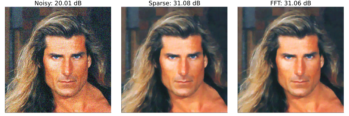
The similarity of results is to be expected because their solving almost exactly the same problem. Where we'll find gains is in our run times.

I ran some rudimentary timing tests on different versions of the Fabio image and hard-coded results in the visualization script below. The FFT version is seriously fast in comparison.

using Plots, StatsPlots
t1 = [3.3, 14.2, 24.5, 101.0] # tvd times
t2 = [0.5, 1.6,  2.8,  10.8]  # tvd_fft times
name = repeat(["Gray 256", "Color 256", "Gray 512", "Color 512"], outer=2)
group= repeat(["Sparse", "FFT"], inner=4)
groupedbar(name, [t1;t2], group=group)
ylabel!("time (s)")
savefig("timebar.svg")

As a last example, I'll demonstrate that TV denoising is not just a trick for synthetically generated noisy images. Below is a real noisy photo of Masa.

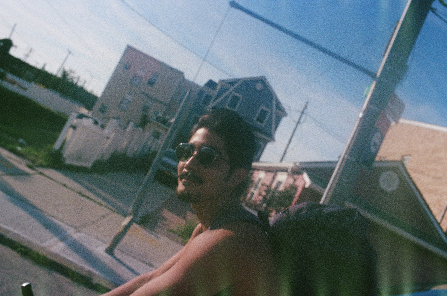
using TVDenoise, FileIO
img = load("masa.png")
x, _ = tvd_fft(img, 0.02, 5)
save("tvdmasa.png", x)

Our TV denoising is able to clean it up nicely.

One question that persists throughout this demos is, "Is there a different set of filters that are better tailored to regularizing the denoising problem?". We can formulate our problem as also being a minimization over $\mathbf{D}$, known as the Analysis Convolutional Dictionary Learning problem. Special care has to be taken to ensure that $\mathbf{D}$ is not degenerate. A Julia implementation for another post!